Population Ecology, part 2
Principles of Ecology Week 3
Reminders
- Weekly activity due tomorrow (Thursday Sept 7th)
- Read Crouse et al. 1987 and answer questions
- List of potential communities of interest due next Friday (Semester Project)
Stage-structured populations

Stage-structured populations

Putting numbers to demographic processes
Putting numbers to demographic processes
- For a population with \(n\) stages, we can capture the demographic transitions in an \(n\mathrm{-by-}n\) matrix.
- Each element captures the contribution from the current column, to the current row.
- The top row always reflects new births
- The first (leftmost) column reflects the youngest individuals
- The last (rightmost) column reflects the oldest individuals
Transition matrix
\[ \begin{bmatrix} ~ & ~ & ~ & ~ & ~& ~ & ~ \\ ~ & ~ & ~ & ~ & ~& ~ & ~ \\ ~ & ~ & ~ & ~ & ~& ~ & ~ \\ ~ & ~ & ~ & ~ & ~& ~ & ~ \\ ~ & ~ & ~ & ~ & ~& ~ & ~ \\ ~ & ~ & ~ & ~ & ~& ~ & ~ \end{bmatrix} \]
Worked example
Consider a species of fish whose individuals live for 3 years (age classes 0, 1, 2, and 3). Newborn fish have a \(30\%\) survival rate to year 1; year 1 fish have a \(80\%\) survival rate to year 2; year 2 fish have a \(50\%\) survival rate to year 3; and all fish die in their third year.
Newborn fish are sexually immature and cannot give birth. Year 1 fish can give birth to \(1\) newborn per year; Year 2 fish can give birth to \(8\) newborns per year; and Year 3 fish can only give birth to \(0.5\) newborns per year.
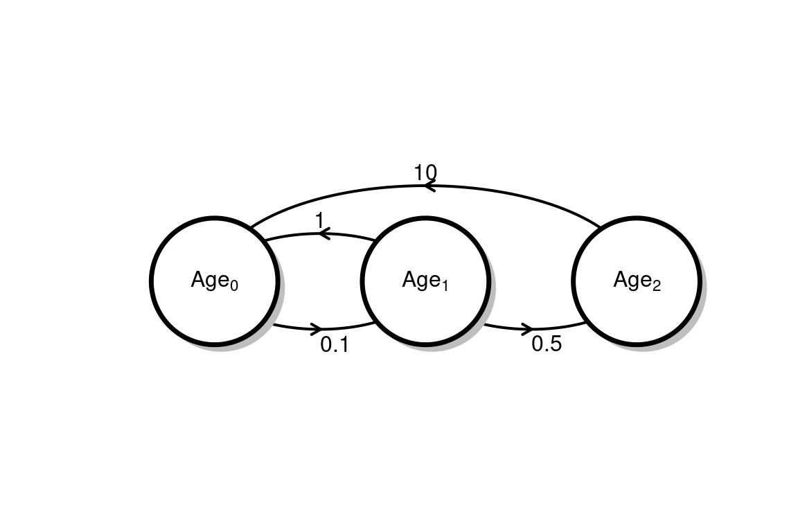
Your task: Draw a life cycle diagram and write the Transition Matrix for this species
The value of a transition matrix
- The product of the current population distribution and the transition matrix tells you the future population distribution
The value of a transition matrix
- From our worked example, recall the transition matrix
\[ \begin{bmatrix} 0 & 1 & 8 & 0.5 \\ 0.3 & 0 & 0 & 0 \\ 0 & 0.8 & 0 & 0 \\ 0 & 0 & 0.5 & 0 \end{bmatrix} \]
At time \(t=0\), the population has \(52\) individuals in stage 0, \(10\) in stage 1, \(15\) in stage 2, and \(30\) in stage 3.
What is the expected distribution of individuals at \(t=1\)?
The value of a transition matrix
Matrix product of the transition matrix and the current distrubition:
\[ \begin{bmatrix} 0 & 1 & 8 & 0.5 \\ 0.3 & 0 & 0 & 0 \\ 0 & 0.8 & 0 & 0 \\ 0 & 0 & 0.5 & 0 \end{bmatrix} \times \begin{bmatrix} 52 \\ 10 \\ 16 \\ 30 \end{bmatrix} \]
The value of a transition matrix
Matrix product of the transition matrix and the current distrubition:
\[ \begin{bmatrix} 0 & 1 & 8 & 0.5 \\ 0.3 & 0 & 0 & 0 \\ 0 & 0.8 & 0 & 0 \\ 0 & 0 & 0.5 & 0 \end{bmatrix} \times \begin{bmatrix} 52 \\ 10 \\ 16 \\ 30 \end{bmatrix} = \begin{bmatrix} 153 \\ 15 \\ 8 \\ 8 \end{bmatrix} \]
The value of a transition matrix
For timestep \(2\):
\[ \begin{bmatrix} 0 & 1 & 8 & 0.5 \\ 0.3 & 0 & 0 & 0 \\ 0 & 0.8 & 0 & 0 \\ 0 & 0 & 0.5 & 0 \end{bmatrix} \times \begin{bmatrix} 153 \\ 15 \\ 8 \\ 8 \end{bmatrix} \]
The value of a transition matrix
For timestep \(2\):
\[ \begin{bmatrix} 0 & 1 & 8 & 0.5 \\ 0.3 & 0 & 0 & 0 \\ 0 & 0.8 & 0 & 0 \\ 0 & 0 & 0.5 & 0 \end{bmatrix} \times \begin{bmatrix} 153 \\ 15 \\ 8 \\ 8 \end{bmatrix} = \begin{bmatrix} 83 \\ 45.9 \\ 12 \\ 4 \end{bmatrix} \]
The value of a transition matrix
For timestep \(3\):
\[ \begin{bmatrix} 0 & 1 & 8 & 0.5 \\ 0.3 & 0 & 0 & 0 \\ 0 & 0.8 & 0 & 0 \\ 0 & 0 & 0.5 & 0 \end{bmatrix} \times \begin{bmatrix} 83 \\ 45.9 \\ 12 \\ 4 \end{bmatrix} = \dots \]
The value of a transition matrix
- We can keep iterating over and over (and over), or….
- Calculate the \(\mathrm{eigenvalue}\) of the transition matrix
- The dominant eigenvalue reflects the long-term growth rate.
\[ \begin{bmatrix} 0 & 1 & 8 & 0.5 \\ 0.3 & 0 & 0 & 0 \\ 0 & 0.8 & 0 & 0 \\ 0 & 0 & 0.5 & 0 \end{bmatrix} \xrightarrow[]{\text{Eigenvalue}} 1.33 \]
The value of a transition matrix
- The dominant Eigenvalue represents the expected long-term annual growth rate (\(\lambda\))
- Populations grow when \(\lambda \gt 1\)
- Populations shrink when \(\lambda \lt 1\)
- Population size is stable when \(\lambda = 1\)
The value of a transition matrix
How is the growth rate affected by particular transitions?
\[ \begin{bmatrix} 0 & 1 & 8 & 0.5 \\ 0.3 & 0 & 0 & 0 \\ 0 & 0.8 & 0 & 0 \\ 0 & 0 & 0.5 & 0 \end{bmatrix} \]
\[ \begin{bmatrix} 0 & 1 & 8 & 0.5 \\ 0.3 \to 0 & 0 & 0 & 0 \\ 0 & 0.8 & 0 & 0 \\ 0 & 0 & 0.5 & 0 \end{bmatrix} \]
\[ \begin{bmatrix} 0 & 1 & 8 & 0.5 \\ 0.3 \to 0.2 & 0 & 0 & 0 \\ 0 & 0.8 & 0 & 0 \\ 0 & 0 & 0.5 & 0 \end{bmatrix} \]
\[ \begin{bmatrix} 0 & 1 & 8 & 0.5 \\ 0.3 \to 0.2 & 0 & 0 & 0 \\ 0 & 0.8 & 0 & 0 \\ 0 & 0 & 0.5 & 0 \end{bmatrix} \Rightarrow \lambda = 1.15 \]
\[ \begin{bmatrix} 0 & 1 & 8 & 0.5 \\ 0.3 & 0 & 0 & 0 \\ 0 & 0.8 \to 0.7 & 0 & 0 \\ 0 & 0 & 0.5 & 0 \end{bmatrix} \]
\[ \begin{bmatrix} 0 & 1 & 8 & 0.5 \\ 0.3 & 0 & 0 & 0 \\ 0 & 0.8 \to 0.7 & 0 & 0 \\ 0 & 0 & 0.5 & 0 \end{bmatrix} \Rightarrow \lambda = 1.28 \]
The value of a transition matrix
How is the growth rate affected by particular transitions?
\[ \begin{bmatrix} 0 & 1 & 8 & 0.5 \\ 0.3 \to 0.2 & 0 & 0 & 0 \\ 0 & 0.8 & 0 & 0 \\ 0 & 0 & 0.5 & 0 \end{bmatrix} \Rightarrow \lambda = 1.15 \]
\[ \begin{bmatrix} 0 & 1 & 8 & 0.5 \\ 0.3 & 0 & 0 & 0 \\ 0 & 0.8 \to 0.7 & 0 & 0 \\ 0 & 0 & 0.5 & 0 \end{bmatrix} \Rightarrow \lambda = 1.28 \]
We can go through each entry one-by-one and identify critical transitions (Sensitivity analysis)
But there is a problem…
Elasticity analysis
Quantify the effects of proportional changes
\[ \begin{bmatrix} 0 & 1 & 8 & 0.5 \\ 0.3 \to 0.27 & 0 & 0 & 0 \\ 0 & 0.8 & 0 & 0 \\ 0 & 0 & 0.5 & 0 \end{bmatrix} \]
\[ \begin{bmatrix} 0 & 1 & 8 & 0.5 \\ 0.3 & 0 & 0 & 0 \\ 0 & 0.8 \to 0.72 & 0 & 0 \\ 0 & 0 & 0.5 & 0 \end{bmatrix} \]
Elasticity analysis
Quantify the effects of proportional changes
\[ \begin{bmatrix} 0 & 1 & 8 & 0.5 \\ 0.3 \to 0.27 & 0 & 0 & 0 \\ 0 & 0.8 & 0 & 0 \\ 0 & 0 & 0.5 & 0 \end{bmatrix} \Rightarrow \lambda=1.28 \]
\[ \begin{bmatrix} 0 & 1 & 8 & 0.5 \\ 0.3 & 0 & 0 & 0 \\ 0 & 0.8 \to 0.72 & 0 & 0 \\ 0 & 0 & 0.5 & 0 \end{bmatrix} \Rightarrow \lambda = 1.29 \]
Principles of Ecology
Week 3, Day 2
Write the transition matrix

Draw a life-cycle diagram
\[ \begin{bmatrix} 0 & 0 & 10 & 1 \\ 0.5 & 0 & 0 & 0 \\ 0 & 0.2 & 0 & 0 \\ 0 & 0 & 0.8 & 0 \end{bmatrix} \]
Transition matrix from Crouse et al. 1987
\[ \begin{bmatrix} 0 & 0 & 0 & 0 & 127 & 4 & 80 \\ 0.67 & 0.74 & 0 & 0 & 0 & 0 & 0 \\ 0 & 0.05 & 0.66 & 0 & 0 & 0 & 0 \\ 0 & 0 & 0.01 & 0.69 & 0 & 0 & 0 \\ 0 & 0 & 0 & 0.05 & 0 & 0 & 0 \\ 0 & 0 & 0 & 0 & 0.81 & 0 & 0 \\ 0 & 0 & 0 & 0 & 0 & 0.81 & 0.81 \\ \end{bmatrix} \]
Translating basic science to action
Why conserve sea turtles?
One, I think they’re important ethically and morally because they’re organisms that have existed on Earth pretty much unchanged for a hundred million or more years, which suggests they do something right. There’s reason to believe that only a few hundred years ago, their populations, say in the Caribbean, were vast – millions and millions of animals. So I think, just ethically and morally, it’s important to conserve them from that point of view.
It appears that there may be a very, very important function from the point of view of transporting nutrients from one part of the oceans to a completely different part of the oceans. Because they are nesting, migrations may come hundreds or even thousands of miles and deposit eggs – all those nutrients that went into making those eggs came from somewhere else. […]
We’re just starting to get hints of what’s going on there.
Review of population ecology models
- Sketch a graph that shows the general shape of a population experiencing exponential growth.
- Sketch a graph that shows the general shape of a population experiencing logistic growth (exponential growth with carrying capacity). Also write the equation for logistic growth.
- What are some biological scenarios when we may want to add a “threshold” for population growth? Name two properties of a system experiencing logistic growth with a threshold.